Archive for January, 2014
Using Real Time Application Metrics To Optimise Solr Indexing Throughput
Posted by Michael Okarimia in 7digital on January 19, 2014
In my previous blog post I wrote about 7digital’s use of real time application monitoring. In this post I will expand upon how the team used application metrics to greatly improve upon a product that powered a critical part of 7digital’s infrastructure.
I’m a member of the Content Discovery Team, who are responsible for making 7digital’s catalogue of 25 million tracks available via the 7digital API.
One of the requirements of making the catalogue accessible is that the lack of a universal unique identifier in music industry that represents artists, tracks and album releases, means that full text searching is important for discovering content. At 7digital, to cope with the increase in both traffic and catalogue size, full text searches were moved over from relational database to Lucene powered Solr database back in 2011
Currently we extract the metadata for the music catalogue from a relational database, transform it to json DTOs and then and post it into our Solr servers, which perform full text searches for music releases, tracks and artists. By placing the catalogue into Solr, this enables it to be searchable, and makes it possible to retrieve releases and artist metadata when supplying a unique 7digital ID.
The datasets are relatively large; creating an index of the entire dataset of 25 million tracks with the schema used would take many days, so it was necessary to append the hourly changes of the catalogue to an existing index.
There was a relational database containing many millions of updates to the catalogue in time order. This was the typical amount of meta-data that is generated per day. Each update would be represented as a single row in a “changes” table in the database.
I.e. a row storing metadata for a track would contain track title, track artist, track price, as some of it’s columns. Each row would have a column denoting if that metadata was being inserted, updated or deleted from the catalogue.
Solr acts as an http wrapper for a Lucene index, so creating an index of the data was done via json posts to the Solr server. One piece of metadata was read from the relational database, mapped into a json document and then posted via HTTP to the Solr server. Solr would then add this document to it’s Lucene index which could be searched. This entire process we refer to as indexing.
The Problem
With the old code base, indexing this data often took hours. This meant that end to end testing in the UAT environment involved lengthy multi hour “code, deploy, run tests” cycles. Typically a change would be made early in the morning so the results could be inspected by lunch time. One could look at the log files to check upon progress, but it became awkward.
The Goal
In early summer 2013 we rewrote the legacy code which performed this Extract, Transform and Load process from the relational database to the Solr server. It was no longer fit for purpose and was causing data inconsistencies which had come about in part from the long feedback cycle between making a code change and seeing the test result.
The goal was improve the metadata indexing throughput to Solr whilst ensuring data correctness. After writing extensive unit and integration tests to verify data consistency, we then turned to performance tuning in our acceptance tests. We wanted to index as many documents to solr as quickly as possible. Log files were available but it wasn’t straightforward to parse meaning from them when looking for patterns across a time span.
This arrangement was clearly suboptimal so we decided to incorporate real-time monitoring. We already were using StatsD to log and Graphite to visualise the web responses on our internal API endpoints and realised we could put it to use to help us here.
After improving the SQL queries, we discovered that the largest factor of indexing throughput was how many documents to post for each commit.
Each document contains a change which could be a delete, an insert or an update of an existing piece of metadata (i.e. a price change of a track). In our scenario, Lucene treats an update and an insert as the same thing; any document indexed that has a matching ID of an existing one will overwrite the original. Changes could therefore be boiled down to either an delete or an “upsert”.
After posting a certain number of documents, a commit command is sent, whereby the index commits the recent changes to disk. Once committed, the new documents are in the index and are searchable. While the commit phase is happening, no new documents can be posted to the Solr server. Depending on the size of the index and the number of documents,the commit phase can take many seconds, or even minutes.
Lucene works effectively when only deletes are committing in one batch and only upserts are committed in another batch. This is much faster than interweaving deletes and upserts within the same period between commits. Commits are when the Lucene index is writing the new documents to the index on the disk, and they come with a minimum time to complete, during which posting new documents is not possible.
Number of rows read mapped directly to the number of documents indexed.
Using the StatsD c# client we counted how long it took to read from the relational database, post the documents to Solr, and then how long it took to commit them, and we sent this timings to a statsD server. We then used Graphite to visualise this data.
The graph below shows:
time taken to read the metadata changes denoting deleted tracks/releases from the relational database, within the given range of rows
time taken to post the delete documents to Solr
time taken for Solr to enact the commit (during which period no new documents may be posted)
time taken to read the metadata changes denoting the upserted tracks/release from the relational database within the table range given range of rows
time taken to post the new documents to Solr
time taken to for Solr to enact the commit (which prevents any new documents from being posted)
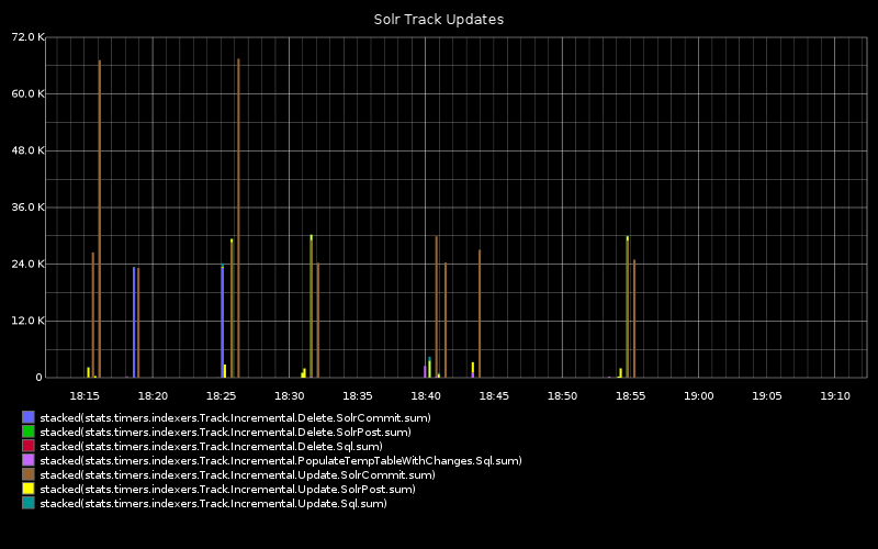
As we can see, commiting updates takes upon 72 seconds and is by far the greatest proportion of time.
Large ranges would make the SQL query component take a long time, occasionally timing out and needing to be repeated. Additionally, commits would take longer.
Using smaller range sizes resulted in more frequent posts and commits to Solr, but commits seemed to have a minimum duration, so there came a point where very small ranges would mean the commit times would be the largest component of the indexing process. and document throughput dropped.
How to measure indexing throughput?
We added some more statsD logging which shows the indexing throughput over the same time period as the chart above.
The below chart shows the row id on the y axis. The each row represents a change of metadata. The blue line shows what is newest change in the relational database. The Green line shows how many of the row ID of the changes that have been posted to Solr. They follow each other with a small delay. A measure of indexing throughput is how closely the green line follows the blue.
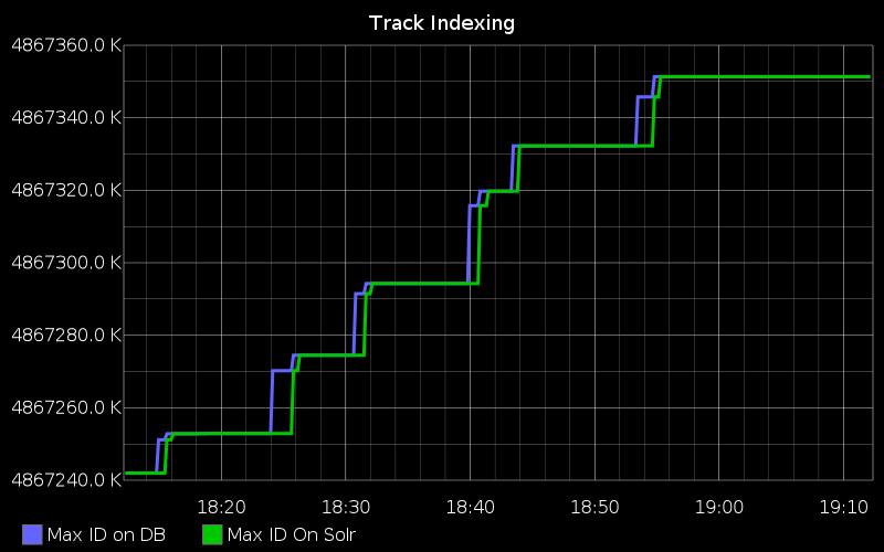
The right of this graph showed us that there were periods of time when no updates are written into the relation database, but when there are writes, the indexer can index them into Solr in less than two minutes
In the C# code that did the Extract, Transform and Load, we added additional statsD metrics, which posted the max rowID of changes table in the relational database, and what the latest rowID that had been posted to Solr. This graph is still used in production to monitor the application in real time. It lets us observe when many metadata changes are made, (for instance, when new content is added) and diagnose any issues with the database we read from, and how long it may take for the content to become available in the Solr servers.
The Result
By being able to monitor how many new changes were being written to the database, and how quickly the indexer can commit it to Solr, we discovered that over a certain rate, increasing throughput would not have a noticeable effect, since there was no benefit in attempting to read more rows per hour than there were being created. This level of monitoring allowed us to effectively decide upon the direction to take when developing the product. The monitoring gave us additional unexpected benefits of having visibility of a business critical database process which was previously unmonitored, the rate of changes recorded was now known.
Ultimately in order to maximise end to end indexing throughout, we found a sweet spot of 100k documents, and by using the the metrics we only optimised where we needed to, thus saving valuable development time.